

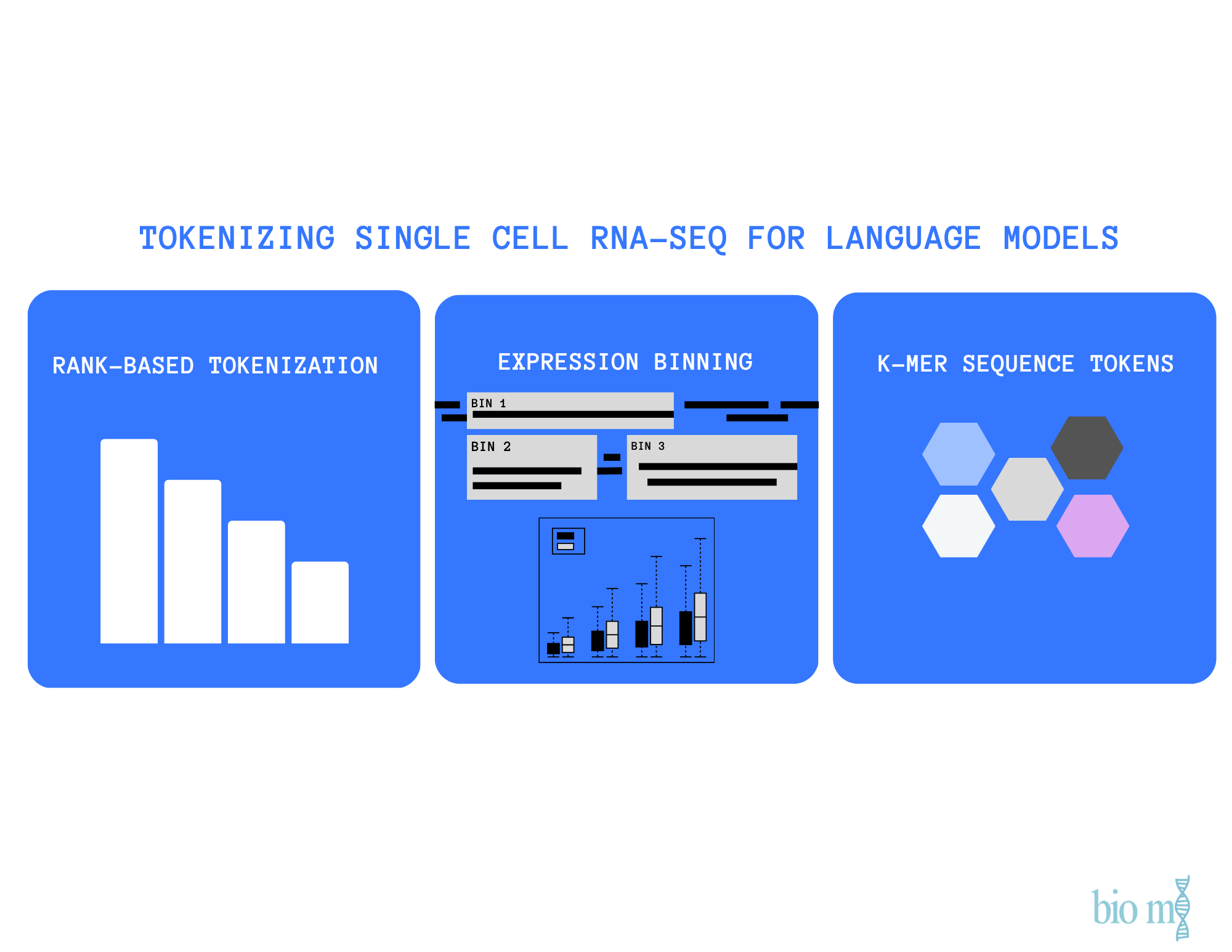
Tokenizing scRNA-seq for Language Models
Comparing k-mers, gene IDs, and learned tokenizations for representing scRNA-seq data in transformer models.
scRNA-seq data measure gene expression across the entire transcriptome of each cell, producing a continuous vector of thousands of expression values per cell. Unlike text, where words naturally form a sequence, gene expression lacks inherent ordering or discrete units.
In traditional natural language processing (NLP), tokenization splits text into discrete symbols, each assigned an ID, allowing models to learn patterns from sequences of tokens.
Classic transformers are built on the assumption that they operate in discrete time and space, processing a sequence of distinct, position-indexed tokens. Vanilla transformers cannot directly ingest raw continuous expression values the way they ingest words.
So the main question becomes:
How can we represent single-cell RNA-seq data as discrete tokens so that transformers can learn from them, as they do from language?
Basic Transformer Processing
Let’s first understand how transformers process inputs…
Inside each layer, every token embedding attends to every other token via pairwise dot-product similarity. Each attention head computes how much information to aggregate from other tokens based on their similarity in embedding space.
In standard language transformers, each input token is an integer ID drawn from a finite vocabulary. This ID indexes a learned embedding matrix E, mapping tokens to continuous vectors:
These token embeddings are stacked row-wise to form an input matrix.
& the embedding vectors are then projected into queries, keys, and values:
Why can’t raw scRNA-seq data be fed directly into a transformer?
Transformers were initially designed for language and operate on the following assumptions:
Input consists of discrete tokens drawn from a fixed vocabulary.
Tokens appear in a well-defined sequence order, encoding through positional embeddings (Vaswani et al., 2017).
Unfortunately, single-cell RNA-seq data violates each of the assumptions.
A cell is typically represented as a continuous, high-dimensional expression vector rather than a sequence of categorical symbols. Important to note that the set of genes holds no inherent positional ordering.
In addition, single-cell foundation models have input dimensionality (i.e ~20k genes) far beyond that of a regular transformer sequence length.
To address this, current single-cell foundation models, such as Geneformer (Theodoris et al., 2023) and scGPT (Cui et al., 2024), employ tokenization frameworks that discretize expression values and propose artificial gene orders to improve data compatibility.
Tokenization Strategies Across Single-Cell Foundation Models
Comparing three different models: Geneformer, scGPT and DNABERT
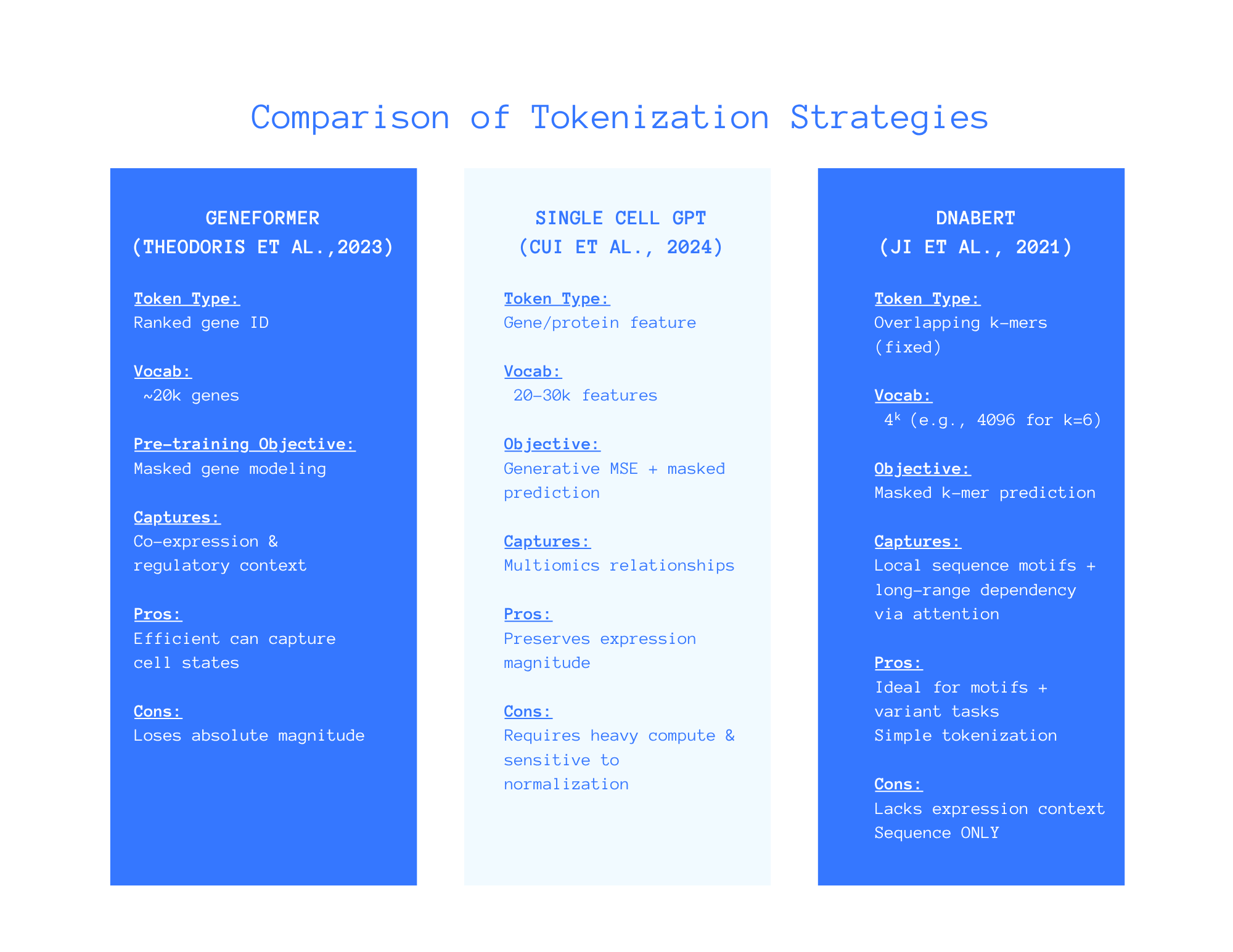
Written comparison of each approach as shown in the above figure.
Geneformer Model (Theodoris et al., 2023)
Token Type: Ranked gene IDs.
Vocab: ~ 20k genes.
Objective: Masked genes.
Captures: Co-expression and regulatory context.
Pros: Efficiently captures cell statistics.
Cons: Loses absolute expression magnitude.
scGPT Model (Cui et al., 2024)
Token Type: Gene/protein features.
Vocab: ~20-30k features.
Objective: Generative means squared error and masked values.
Captures: Multiomic relationships (i.e RNA, ATAC, proteins).
Pros: Preserves expression magnitude.
Cons: Requires heavy computing & is sensitive to normalization.
DNABERT (Ji et al., 2021)
Token Type: Overlapping k-mers (fixed).
Vocab: 4ᵏ (e.g., 4096 for k=6)
Objective: Masked k-mer prediction.
Captures: Local sequence motifs & long-range dependency via attention.
Pros: Ideal for motifs and variant tasks.
Cons: Lacks expression context and is sequence ONLY.
Geneformer Model Breakdown
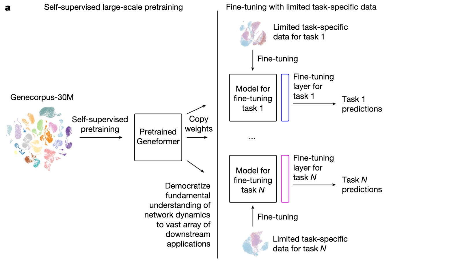
Geneformer utilizes the transformer architecture for single-cell transcriptomes. It represents each cell as a ranked list of gene tokens, ordered by expression level. Through pretraining, the model learns co-expression and regulatory relationships by predicting masked genes based on their surrounding gene context.
In this objective, gj represents a masked gene, and P(gj | context) is the probability that the model correctly predicts it based on the other expressed genes in the same cell.
Only a small portion of genes were masked —approximately 15% in each transcriptome (Theodoris et al., 2023). Inspired by BERT language models, helps balance prediction difficulty with information retention during pretraining.
By optimizing the masked prediction task, Geneformer builds a latent representation that reflects how genes interact across regulatory networks— gaining a deeper understanding of how each relative ranking encodes across states of differentiation and disease.
Geneformer uses in-silico perturbations to simulate gene knockouts by removing a specific gene token and evaluating how the cell’s embedding changes. A variation in the cell’s embedding space provides a prediction towards the eventual functional impact of a gene.
Here, Eorig and Edeleted are the embeddings of the same cell before gene knockouts. A larger cosine distance (∆s) indicates that deleting a gene substantially alters the cell’s overall transcriptomic state, suggesting a greater influence of functional significance. Ensuring Geneformer can approximate experimental perturbations computationally.
scGPT Model Breakdown
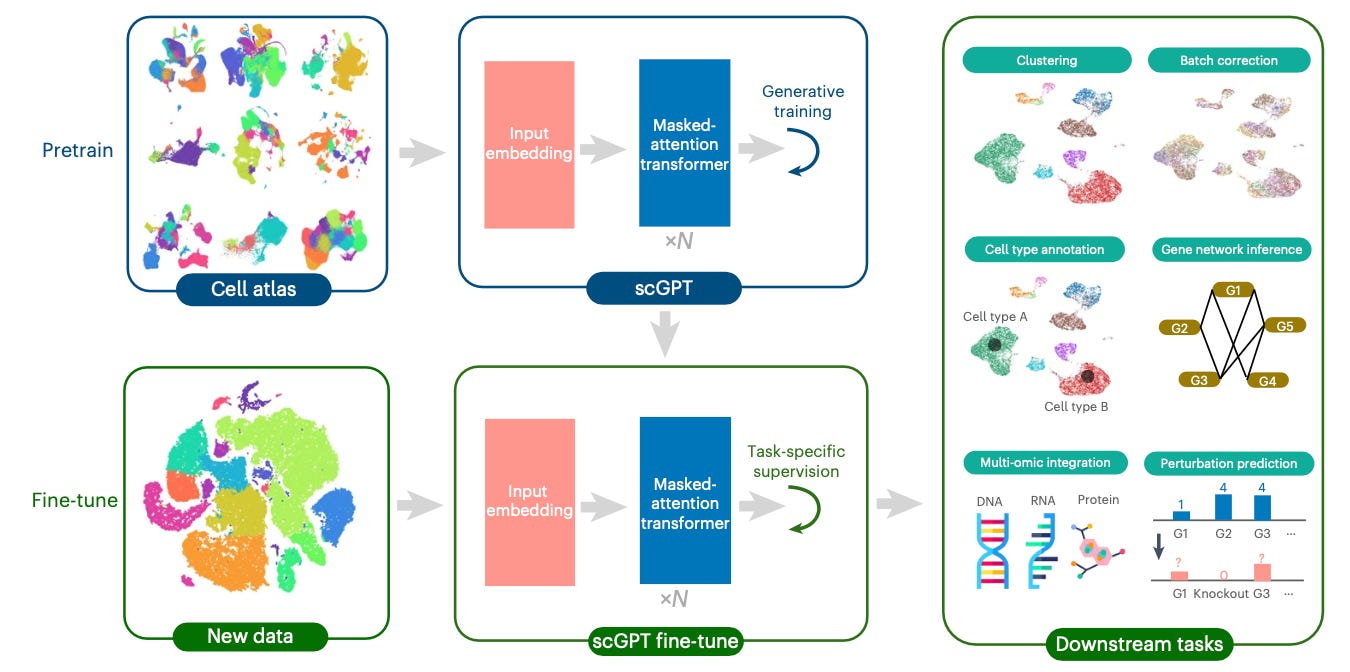
scGPT extends to single-cell multi-omics data by learning relationships among molecular features, such as genes and proteins. Each gene token attends to others through scaled dot-prediction attention.
scGPT then uses this information to identify reliance on molecular features within and across modalities. For example, linking gene-expression signals from scRNA-seq with chromatin-accessibility patterns from scATAC-seq or protein levels from CITE-seq.
Here, Q, K, and V are linear projections of the input embeddings, and d is the feature dimension used to stabilize scaling. The softmax operation converts similarities from the genes pretraining to attention weights to evaluate how heavily a feature would contribute to another’s representation.
As pretraining proceeds, gene or protein features are divided into subsets and masked so the model can learn to reconstruct them from the remaining context. As opposed to predicting pretraining labels, scGPT predicts continuous expression values (i.e generative task).
Therefore, the subsequent pretraining loss is calculated from the MSE between predicted and actual values of the masked features of the models equation.
U_unk represents the set of masked features, x_j is the actual expression value, and x & j the model’s prediction. By minimizing L_gen, scGPT pretrains molecular information from partial observations, much as a language model predicts missing words.
Once pretraining concludes, scGPT can adapt to specific biological tasks, such as predicting cell types, perturbation responses, and more. Fine-tuning combines a task-specific loss with the generative objective to maintain the pretrained representations.
Here, the Ltask measures performance on the downstream problem, while the regularization term λLgen maintains generative consistency.
When combined, this allows scGPT to transfer and apply the cellular learnings to new experimental conditions.
DNABERT Model Breakdown
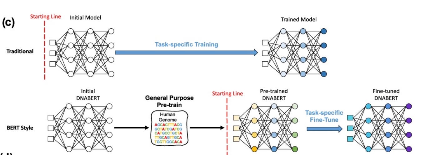
DNABERT treats DNA as a sequence of overlapping k-mers. Each k-mer is embedded into a continuous vector Et and combined with its positional encoding It to form the input matrix M.
This equation defines DNABERT’s self-attention mechanism, used in each transformer head. The matrices Wi^Q, Wi^K and Wi^V are learned projections that transform the input M into query, key and value representations.
The dot product between queries and keys measures the similarity between k-mers, scaled by √dk and normalized using softmax. After normalization, we produce attention weights, which are then applied to values to generate context-aware representations.
Outputs from multiple attention heads are concatenated and linearly transformed using W^O. Each head captures unique information about sequence-element relations, ultimately allowing DNABERT to model both local and long-range dependencies across the genome.
During pre-training, 15% of contiguous k-mers are randomly masked and predicted from their surrounding sequence context, following the self-supervised setup introduced by Ji et al. (2021).
The model minimizes cross-entropy loss, L, where y’i is the actual label for each masked k-mer and yi is the predicted probability. The objective enables DNABERT to learn the structure and semantics of genomic sequences before fine-tuning on specific downstream tasks.
Limitations of Transformer Tokenization for scRNA-seq
1. Loss of magnitude information
As mentioned previously in this article, it should come as no surprise that transformers require discrete tokens. As a result, many single-cell models collapse continuous expression values into categorical representations. Geneformer highlights this by replacing raw transcript counts with rank value encodings, acknowledging that absolute expression magnitudes are discarded.
The authors state that genes are “stored as ranked tokens as opposed to exact transcript values” (Theodoris et al., 2023). Ultimately, allowing transformers to operate and obscure subtle differences in gene dosage, weak regulatory signals or nuanced differential expression patterns.
Lowly expressed but high-information genes (e.g., TFs, cytokines, lineage-specifying regulators) often fall below the top-2048 cutoff and are removed from the discrete sequence, thereby eliminating key biological signals.
2. Sequence length constraints
Transformers scale quadratically with sequence length (O(L²), making it infeasible to process a complete ~20,000-gene scRNA-seq profile.
Geneformer confronts this directly by truncating each cell to the top 2,048 genes because “input size of 2,048… represents 93% of rank value encodings” and was the maximum manageable length (Theodoris et al., 2023).
DNABERT also reinforces a similar principle in sequence modelling, restricting input sequences to a maximum length of 512 tokens (Ji et al., 2021). These examples support the same takeaway message that transformer models can only examine a small subset of each cell’s transcriptome.
*Note: Quadratic attention means 20k x 20k attention = 400M pairwise interactions per’cell
3. Vocabulary size trade-offs
Tokenization imposes biological features on a discrete vocabulary. In biology, the term 'vocabulary' is arbitrary, since we don’t necessarily have a canonical alphabet. For models operating on sequences, k-mer tokenization leads to exponential growth in vocabulary size.
For example, in DNABERT, “there are 4^k + 5 tokens in the vocabulary” (Ji et al., 2021, 2114). For gene-based models such as Geneformer or scGPT, the vocabulary size will be bounded by the number of detectable genes (~20- 25k).
Larger vocabularies can improve expressivity but increase embedding-layer memory usage, sparsity, and training instability.
Fixed vocabularies are often brittle across datasets, whereas large vocabularies have better biological coverage but struggle with optimization. From my understanding, most current models lack “biologically learned vocabularies”.
4. Cross-dataset & cross-species generalization
The majority of tokenization workflows are grounded in specific vocabulary, gene index ordering, or dataset distribution, as opposed to natural languages, where biological “vocabularies” differ across datasets, tissues and species.
DNABERT demonstrates this explicitly: although 85% of protein-coding regions are orthologous between human and mouse, non-coding regions show only ~50% similarity (Ji et al., 2021, 2117), which undermines the stability of k-mer vocabularies across species.
Gene ID tokenizers can fail if the genes do not map cleanly between organisms.
Rank-based tokenizers also tend to depend on dataset-specific gene detection rates.
Overall, generalizing pretrained embeddings across organisms or sequencing platforms remains problematic.
5. Objective Mismatch
Large language models primarily rely on masking or the prediction of discrete tokens to predict the next word. With continuous values, there’s no vocab to mask or predict symbolically loss functions like cross entropy on discrete IDs, which no longer apply.
As seen in scGPT (Cui et al., 2024), the loss function is the mean squared error (MSE), which quantifies the numerical difference between a predicted continuous value and the ground-truth continuous value.
Transformers rely on discrete next-token prediction to scale. Continuous regression (MSE) does not benefit from the typical scaling laws that LLMs rely on.
Conclusion
Tokenization defines the interface between scRNA-seq and transformers. Each approach makes different assumptions about biological structure, and these assumptions determine what the model can ultimately learn.
As single-cell foundation models expand, improving tokenization will be crucial for capturing richer variation and making biologically meaningful predictions.
Thanks for reading :)
I (Lauren) started this blog to serve as an digital lab notebook; a place to support my development as an lifelong learner and growing researcher in CS + bio.
P.S: I’m still learning, experimenting, and figuring out how all these pieces fit together. If you have feedback, ideas, or things I should explore next, I’d genuinely appreciate it.
References
Cui, H., Wang, C., Maan, H., Pang, K., Luo, F., Duan, N., & Wang, B. (2024). scGPT: toward building a foundation model for single cell multi-omics using generative AI. Nature Methods, 21, 1470-1480. https://www.nature.com/articles/s41592-024-02201-0
Ji, Y., Zhou, Z., Liu, H., & Davuluri, R. V. (2021, August). DNABERT: pre-trained Bidirectional Encoder Representations from Transformers model for DNA-language in genome. Bioinformatics, 37(15), 2112-2120. Oxford University Press. https://doi.org/10.1093/bioinformatics/btab083
Theodoris, C. V., Zeng, Z., & Liu, S. (2023). Transfer Learning enables predictions in network biology. Nature, 618, 616-624. https://doi.org/10.1038/s41586-023-06139-9
Vaswani, A., Shazeer, N., Parmar, N., Uszkoreit, J., Jones, L., Gomez, A. N., Kaiser, L., & Polosukhin, I. (2017). Attention Is All You Need. arXiv, arXiv:1706.03762 [cs.CL]. Retrieved 2025, from https://arxiv.org/pdf/1706.03762
love how u included the equations as well!! great first article!